Hyperliquid Vault PnL Analysis
In this notebook, we demonstrate how to analyse the historical performance of a Hyperliquid vault by reconstructing its position history and visualising the equity curve (cumulative PnL).
What we’ll cover:
Fetching trade fills from Hyperliquid API for a specific vault
Reconstructing position events (opens, closes, increases, decreases) from fill data
Creating an analysis DataFrame with exposure and PnL tracking per market
Visualising the vault’s equity curve using Plotly
Analysing vault deposits and withdrawals (capital flows)
Combining PnL and deposits to visualise overall account value
Calculating internal share price to measure true investment performance
About Hyperliquid Vaults:
Hyperliquid vaults are managed trading accounts where depositors delegate capital to vault managers who execute perpetual futures trading strategies. Unlike ERC-4626 vaults, Hyperliquid vaults operate natively on Hyperliquid Core, a specialised chain that is not EVM compatible.
Note: The Hyperliquid API has pagination limits (max 10,000 fills), so historical analysis is limited to recent trading activity.
For questions or feedback, contact Trading Strategy community.
Setup
Configure notebook display settings
Set up Plotly for static image output (for documentation rendering)
[29]:
import datetime
import pandas as pd
from plotly.offline import init_notebook_mode
import plotly.io as pio
import plotly.graph_objects as go
pd.options.display.float_format = "{:,.2f}".format
pd.options.display.max_columns = None
pd.options.display.max_rows = None
# Set up Plotly chart output
image_format = "png"
width = 1200
height = 600
init_notebook_mode()
pio.renderers.default = image_format
current_renderer = pio.renderers[image_format]
current_renderer.width = width
current_renderer.height = height
Vault Configuration
We’ll analyze the Trading Strategy - IchiV3 LS vault, which executes long/short perpetual futures strategies.
You can view this vault on the Hyperliquid app: https://app.hyperliquid.xyz/vaults/0x3df9769bbbb335340872f01d8157c779d73c6ed0
[30]:
# Vault address to analyze
VAULT_ADDRESS = "0x3df9769bbbb335340872f01d8157c779d73c6ed0"
# Time range for analysis (last 30 days by default)
END_TIME = datetime.datetime.now()
START_TIME = END_TIME - datetime.timedelta(days=30)
# Display configuration as a table
config_df = pd.DataFrame({
"Setting": ["Vault Address", "Start Date", "End Date"],
"Value": [VAULT_ADDRESS, START_TIME.strftime('%Y-%m-%d'), END_TIME.strftime('%Y-%m-%d')]
})
display(config_df.set_index("Setting"))
| Value | |
|---|---|
| Setting | |
| Vault Address | 0x3df9769bbbb335340872f01d8157c779d73c6ed0 |
| Start Date | 2025-11-30 |
| End Date | 2025-12-30 |
Fetch Trade Fills
First, we create an HTTP session configured with retry logic for the Hyperliquid API, then fetch all trade fills for the vault within our time range.
The API returns fills in reverse chronological order, but our fetch function automatically sorts them chronologically for position reconstruction.
[31]:
from eth_defi.hyperliquid.session import create_hyperliquid_session
from eth_defi.hyperliquid.position import fetch_vault_fills
# Create session with automatic retry logic
session = create_hyperliquid_session()
# Fetch fills for the vault
fills = list(fetch_vault_fills(
session,
VAULT_ADDRESS,
start_time=START_TIME,
end_time=END_TIME,
))
print(f"Fetched {len(fills)} fills")
# Show sample fills as a table
if fills:
sample_data = []
for fill in fills[:5]: # Show first 5 fills
sample_data.append({
"Coin": fill.coin,
"Side": fill.side,
"Size": float(fill.size),
"Price": float(fill.price),
"Time": fill.timestamp,
})
display(pd.DataFrame(sample_data))
Fetched 128 fills
| Coin | Side | Size | Price | Time | |
|---|---|---|---|---|---|
| 0 | ENA | B | 107.00 | 0.24 | 2025-12-01 06:07:19.756 |
| 1 | WLFI | B | 205.00 | 0.15 | 2025-12-02 11:01:08.209 |
| 2 | XRP | B | 23.00 | 2.19 | 2025-12-03 22:05:03.025 |
| 3 | ADA | A | 92.00 | 0.45 | 2025-12-04 01:01:07.787 |
| 4 | WLFI | A | 205.00 | 0.16 | 2025-12-04 18:01:21.837 |
Reconstruct Position History
The raw fills don’t directly tell us about position state. We need to process them chronologically to reconstruct position events:
Open: New position from flat
Close: Position closed to flat (realised PnL)
Increase: Position size increased
Decrease: Partial position reduction (realised PnL)
[32]:
from eth_defi.hyperliquid.position import reconstruct_position_history, get_position_summary
# Reconstruct position events from fills
events = list(reconstruct_position_history(fills))
print(f"Reconstructed {len(events)} position events")
# Show position summary per market as a table
summary = get_position_summary(events)
summary_data = []
for coin, stats in sorted(summary.items()):
summary_data.append({
"Market": coin,
"Total Trades": stats['total_trades'],
"Opens": stats['opens'],
"Closes": stats['closes'],
"Realised PnL": float(stats['total_realized_pnl']),
"Total Fees": float(stats['total_fees']),
})
summary_df = pd.DataFrame(summary_data).set_index("Market")
display(summary_df)
Reconstructed 129 position events
| Total Trades | Opens | Closes | Realised PnL | Total Fees | |
|---|---|---|---|---|---|
| Market | |||||
| 0G | 7 | 1 | 1 | 0.76 | 0.59 |
| AAVE | 4 | 1 | 1 | 96.61 | 0.66 |
| ACE | 13 | 5 | 5 | -125.76 | 2.42 |
| ADA | 2 | 1 | 1 | -1.87 | 0.04 |
| APEX | 2 | 1 | 1 | -3.02 | 0.04 |
| APT | 2 | 1 | 1 | -30.65 | 0.64 |
| ARB | 2 | 1 | 1 | -0.98 | 0.02 |
| AVNT | 6 | 1 | 1 | -75.53 | 0.69 |
| BTC | 3 | 2 | 1 | -0.40 | 0.37 |
| CC | 3 | 1 | 1 | -16.09 | 0.25 |
| CRV | 2 | 1 | 1 | 0.49 | 0.02 |
| DOGE | 2 | 1 | 1 | 1.07 | 0.02 |
| ENA | 1 | 1 | 0 | 0.00 | 0.01 |
| HBAR | 2 | 1 | 1 | 2.63 | 0.01 |
| HYPE | 5 | 2 | 1 | 0.00 | 0.28 |
| LDO | 4 | 1 | 1 | -5.77 | 0.23 |
| LTC | 3 | 1 | 0 | 0.00 | 0.41 |
| MERL | 5 | 1 | 1 | -33.83 | 0.64 |
| MON | 7 | 2 | 1 | -48.90 | 0.96 |
| SEI | 2 | 1 | 1 | -0.52 | 0.02 |
| SUI | 2 | 1 | 1 | 0.86 | 0.03 |
| TAO | 2 | 1 | 1 | -0.87 | 0.02 |
| TRX | 4 | 2 | 2 | -2.91 | 0.23 |
| USTC | 2 | 1 | 1 | -1.43 | 0.02 |
| VVV | 8 | 2 | 1 | 32.01 | 0.96 |
| WIF | 1 | 1 | 0 | 0.00 | 0.05 |
| WLD | 2 | 1 | 1 | 0.58 | 0.02 |
| WLFI | 8 | 3 | 3 | -10.09 | 0.31 |
| XPL | 4 | 1 | 1 | -13.63 | 0.24 |
| XRP | 4 | 1 | 0 | -2.51 | 0.07 |
| ZEC | 13 | 4 | 4 | 249.09 | 2.18 |
| ZORA | 2 | 1 | 1 | 1.53 | 0.02 |
Create Analysis DataFrame
Now we convert the position events into a pandas DataFrame suitable for analysis. The DataFrame tracks:
Exposure: Notional value (size × price) for each position direction per market
PnL: Cumulative realised profit/loss for each direction per market
Column naming convention: - {coin}_long_exposure / {coin}_long_pnl - {coin}_short_exposure / {coin}_short_pnl
[33]:
from eth_defi.hyperliquid.position_analysis import create_account_dataframe
# Create the analysis DataFrame
df = create_account_dataframe(events)
# Display DataFrame info as a table
info_df = pd.DataFrame({
"Metric": ["Rows", "Columns", "Start Time", "End Time"],
"Value": [df.shape[0], df.shape[1], str(df.index.min()), str(df.index.max())]
})
display(info_df.set_index("Metric"))
# Show the last few rows
display(df.tail())
| Value | |
|---|---|
| Metric | |
| Rows | 129 |
| Columns | 128 |
| Start Time | 2025-12-01 06:07:19.756000 |
| End Time | 2025-12-29 20:07:28.020000 |
| 0G_long_exposure | 0G_long_pnl | 0G_short_exposure | 0G_short_pnl | AAVE_long_exposure | AAVE_long_pnl | AAVE_short_exposure | AAVE_short_pnl | ACE_long_exposure | ACE_long_pnl | ACE_short_exposure | ACE_short_pnl | ADA_long_exposure | ADA_long_pnl | ADA_short_exposure | ADA_short_pnl | APEX_long_exposure | APEX_long_pnl | APEX_short_exposure | APEX_short_pnl | APT_long_exposure | APT_long_pnl | APT_short_exposure | APT_short_pnl | ARB_long_exposure | ARB_long_pnl | ARB_short_exposure | ARB_short_pnl | AVNT_long_exposure | AVNT_long_pnl | AVNT_short_exposure | AVNT_short_pnl | BTC_long_exposure | BTC_long_pnl | BTC_short_exposure | BTC_short_pnl | CC_long_exposure | CC_long_pnl | CC_short_exposure | CC_short_pnl | CRV_long_exposure | CRV_long_pnl | CRV_short_exposure | CRV_short_pnl | DOGE_long_exposure | DOGE_long_pnl | DOGE_short_exposure | DOGE_short_pnl | ENA_long_exposure | ENA_long_pnl | ENA_short_exposure | ENA_short_pnl | HBAR_long_exposure | HBAR_long_pnl | HBAR_short_exposure | HBAR_short_pnl | HYPE_long_exposure | HYPE_long_pnl | HYPE_short_exposure | HYPE_short_pnl | LDO_long_exposure | LDO_long_pnl | LDO_short_exposure | LDO_short_pnl | LTC_long_exposure | LTC_long_pnl | LTC_short_exposure | LTC_short_pnl | MERL_long_exposure | MERL_long_pnl | MERL_short_exposure | MERL_short_pnl | MON_long_exposure | MON_long_pnl | MON_short_exposure | MON_short_pnl | SEI_long_exposure | SEI_long_pnl | SEI_short_exposure | SEI_short_pnl | SUI_long_exposure | SUI_long_pnl | SUI_short_exposure | SUI_short_pnl | TAO_long_exposure | TAO_long_pnl | TAO_short_exposure | TAO_short_pnl | TRX_long_exposure | TRX_long_pnl | TRX_short_exposure | TRX_short_pnl | USTC_long_exposure | USTC_long_pnl | USTC_short_exposure | USTC_short_pnl | VVV_long_exposure | VVV_long_pnl | VVV_short_exposure | VVV_short_pnl | WIF_long_exposure | WIF_long_pnl | WIF_short_exposure | WIF_short_pnl | WLD_long_exposure | WLD_long_pnl | WLD_short_exposure | WLD_short_pnl | WLFI_long_exposure | WLFI_long_pnl | WLFI_short_exposure | WLFI_short_pnl | XPL_long_exposure | XPL_long_pnl | XPL_short_exposure | XPL_short_pnl | XRP_long_exposure | XRP_long_pnl | XRP_short_exposure | XRP_short_pnl | ZEC_long_exposure | ZEC_long_pnl | ZEC_short_exposure | ZEC_short_pnl | ZORA_long_exposure | ZORA_long_pnl | ZORA_short_exposure | ZORA_short_pnl | |
|---|---|---|---|---|---|---|---|---|---|---|---|---|---|---|---|---|---|---|---|---|---|---|---|---|---|---|---|---|---|---|---|---|---|---|---|---|---|---|---|---|---|---|---|---|---|---|---|---|---|---|---|---|---|---|---|---|---|---|---|---|---|---|---|---|---|---|---|---|---|---|---|---|---|---|---|---|---|---|---|---|---|---|---|---|---|---|---|---|---|---|---|---|---|---|---|---|---|---|---|---|---|---|---|---|---|---|---|---|---|---|---|---|---|---|---|---|---|---|---|---|---|---|---|---|---|---|---|---|
| timestamp | ||||||||||||||||||||||||||||||||||||||||||||||||||||||||||||||||||||||||||||||||||||||||||||||||||||||||||||||||||||||||||||||||
| 2025-12-29 13:05:31.428 | 0.00 | 0.76 | 0.00 | 0.00 | 0.00 | 0.00 | 0.00 | 96.61 | 0.00 | -18.65 | 0.00 | -107.11 | 0.00 | 0.00 | 0.00 | -1.87 | 0.00 | 0.00 | 0.00 | -3.02 | 0.00 | 0.00 | 0.00 | -30.65 | 0.00 | 0.00 | 0.00 | -0.98 | 0.00 | 0.00 | 0.00 | -75.53 | 0.00 | -0.40 | 773.20 | 0.00 | 0.00 | -16.09 | 0.00 | 0.00 | 0.00 | 0.00 | 0.00 | 0.49 | 0.00 | 0.00 | 0.00 | 1.07 | 26.09 | 0.00 | 0.00 | 0.00 | 0.00 | 0.00 | 0.00 | 2.63 | 18.81 | 0.00 | 0.00 | 0.00 | 0.00 | 0.00 | 0.00 | -5.77 | 0.00 | 0.00 | 908.15 | 0.00 | 0.00 | -33.83 | 0.00 | 0.00 | 0.00 | 0.00 | 712.96 | -48.90 | 0.00 | -0.52 | 0.00 | 0.00 | 0.00 | 0.86 | 0.00 | 0.00 | 0.00 | -0.87 | 0.00 | 0.00 | 0.00 | -0.07 | 0.00 | -2.84 | 0.00 | -1.43 | 0.00 | 0.00 | 689.13 | 32.01 | 0.00 | 0.00 | 0.00 | 0.00 | 116.52 | 0.00 | 0.00 | 0.00 | 0.00 | 0.58 | 0.00 | -0.17 | 0.00 | -9.92 | 0.00 | 0.00 | 0.00 | -13.63 | 47.55 | -2.51 | 0.00 | 0.00 | 0.00 | 226.89 | 0.00 | 22.20 | 0.00 | 0.00 | 0.00 | 1.53 |
| 2025-12-29 20:07:28.020 | 0.00 | 0.76 | 0.00 | 0.00 | 0.00 | 0.00 | 0.00 | 96.61 | 0.00 | -18.65 | 0.00 | -107.11 | 0.00 | 0.00 | 0.00 | -1.87 | 0.00 | 0.00 | 0.00 | -3.02 | 0.00 | 0.00 | 0.00 | -30.65 | 0.00 | 0.00 | 0.00 | -0.98 | 0.00 | 0.00 | 0.00 | -75.53 | 0.00 | -0.40 | 773.20 | 0.00 | 0.00 | -16.09 | 0.00 | 0.00 | 0.00 | 0.00 | 0.00 | 0.49 | 0.00 | 0.00 | 0.00 | 1.07 | 26.09 | 0.00 | 0.00 | 0.00 | 0.00 | 0.00 | 0.00 | 2.63 | 0.00 | 0.00 | 0.00 | 0.00 | 0.00 | 0.00 | 0.00 | -5.77 | 0.00 | 0.00 | 908.15 | 0.00 | 0.00 | -33.83 | 0.00 | 0.00 | 0.00 | 0.00 | 712.96 | -48.90 | 0.00 | -0.52 | 0.00 | 0.00 | 0.00 | 0.86 | 0.00 | 0.00 | 0.00 | -0.87 | 0.00 | 0.00 | 0.00 | -0.07 | 0.00 | -2.84 | 0.00 | -1.43 | 0.00 | 0.00 | 689.13 | 32.01 | 0.00 | 0.00 | 0.00 | 0.00 | 116.52 | 0.00 | 0.00 | 0.00 | 0.00 | 0.58 | 0.00 | -0.17 | 0.00 | -9.92 | 0.00 | 0.00 | 0.00 | -13.63 | 47.55 | -2.51 | 0.00 | 0.00 | 0.00 | 226.89 | 0.00 | 22.20 | 0.00 | 0.00 | 0.00 | 1.53 |
| 2025-12-29 20:07:28.020 | 0.00 | 0.76 | 0.00 | 0.00 | 0.00 | 0.00 | 0.00 | 96.61 | 0.00 | -18.65 | 0.00 | -107.11 | 0.00 | 0.00 | 0.00 | -1.87 | 0.00 | 0.00 | 0.00 | -3.02 | 0.00 | 0.00 | 0.00 | -30.65 | 0.00 | 0.00 | 0.00 | -0.98 | 0.00 | 0.00 | 0.00 | -75.53 | 0.00 | -0.40 | 773.20 | 0.00 | 0.00 | -16.09 | 0.00 | 0.00 | 0.00 | 0.00 | 0.00 | 0.49 | 0.00 | 0.00 | 0.00 | 1.07 | 26.09 | 0.00 | 0.00 | 0.00 | 0.00 | 0.00 | 0.00 | 2.63 | 0.00 | 0.00 | 27.13 | 0.00 | 0.00 | 0.00 | 0.00 | -5.77 | 0.00 | 0.00 | 908.15 | 0.00 | 0.00 | -33.83 | 0.00 | 0.00 | 0.00 | 0.00 | 712.96 | -48.90 | 0.00 | -0.52 | 0.00 | 0.00 | 0.00 | 0.86 | 0.00 | 0.00 | 0.00 | -0.87 | 0.00 | 0.00 | 0.00 | -0.07 | 0.00 | -2.84 | 0.00 | -1.43 | 0.00 | 0.00 | 689.13 | 32.01 | 0.00 | 0.00 | 0.00 | 0.00 | 116.52 | 0.00 | 0.00 | 0.00 | 0.00 | 0.58 | 0.00 | -0.17 | 0.00 | -9.92 | 0.00 | 0.00 | 0.00 | -13.63 | 47.55 | -2.51 | 0.00 | 0.00 | 0.00 | 226.89 | 0.00 | 22.20 | 0.00 | 0.00 | 0.00 | 1.53 |
| 2025-12-29 20:07:28.020 | 0.00 | 0.76 | 0.00 | 0.00 | 0.00 | 0.00 | 0.00 | 96.61 | 0.00 | -18.65 | 0.00 | -107.11 | 0.00 | 0.00 | 0.00 | -1.87 | 0.00 | 0.00 | 0.00 | -3.02 | 0.00 | 0.00 | 0.00 | -30.65 | 0.00 | 0.00 | 0.00 | -0.98 | 0.00 | 0.00 | 0.00 | -75.53 | 0.00 | -0.40 | 773.20 | 0.00 | 0.00 | -16.09 | 0.00 | 0.00 | 0.00 | 0.00 | 0.00 | 0.49 | 0.00 | 0.00 | 0.00 | 1.07 | 26.09 | 0.00 | 0.00 | 0.00 | 0.00 | 0.00 | 0.00 | 2.63 | 0.00 | 0.00 | 73.30 | 0.00 | 0.00 | 0.00 | 0.00 | -5.77 | 0.00 | 0.00 | 908.15 | 0.00 | 0.00 | -33.83 | 0.00 | 0.00 | 0.00 | 0.00 | 712.96 | -48.90 | 0.00 | -0.52 | 0.00 | 0.00 | 0.00 | 0.86 | 0.00 | 0.00 | 0.00 | -0.87 | 0.00 | 0.00 | 0.00 | -0.07 | 0.00 | -2.84 | 0.00 | -1.43 | 0.00 | 0.00 | 689.13 | 32.01 | 0.00 | 0.00 | 0.00 | 0.00 | 116.52 | 0.00 | 0.00 | 0.00 | 0.00 | 0.58 | 0.00 | -0.17 | 0.00 | -9.92 | 0.00 | 0.00 | 0.00 | -13.63 | 47.55 | -2.51 | 0.00 | 0.00 | 0.00 | 226.89 | 0.00 | 22.20 | 0.00 | 0.00 | 0.00 | 1.53 |
| 2025-12-29 20:07:28.020 | 0.00 | 0.76 | 0.00 | 0.00 | 0.00 | 0.00 | 0.00 | 96.61 | 0.00 | -18.65 | 0.00 | -107.11 | 0.00 | 0.00 | 0.00 | -1.87 | 0.00 | 0.00 | 0.00 | -3.02 | 0.00 | 0.00 | 0.00 | -30.65 | 0.00 | 0.00 | 0.00 | -0.98 | 0.00 | 0.00 | 0.00 | -75.53 | 0.00 | -0.40 | 773.20 | 0.00 | 0.00 | -16.09 | 0.00 | 0.00 | 0.00 | 0.00 | 0.00 | 0.49 | 0.00 | 0.00 | 0.00 | 1.07 | 26.09 | 0.00 | 0.00 | 0.00 | 0.00 | 0.00 | 0.00 | 2.63 | 0.00 | 0.00 | 535.20 | 0.00 | 0.00 | 0.00 | 0.00 | -5.77 | 0.00 | 0.00 | 908.15 | 0.00 | 0.00 | -33.83 | 0.00 | 0.00 | 0.00 | 0.00 | 712.96 | -48.90 | 0.00 | -0.52 | 0.00 | 0.00 | 0.00 | 0.86 | 0.00 | 0.00 | 0.00 | -0.87 | 0.00 | 0.00 | 0.00 | -0.07 | 0.00 | -2.84 | 0.00 | -1.43 | 0.00 | 0.00 | 689.13 | 32.01 | 0.00 | 0.00 | 0.00 | 0.00 | 116.52 | 0.00 | 0.00 | 0.00 | 0.00 | 0.58 | 0.00 | -0.17 | 0.00 | -9.92 | 0.00 | 0.00 | 0.00 | -13.63 | 47.55 | -2.51 | 0.00 | 0.00 | 0.00 | 226.89 | 0.00 | 22.20 | 0.00 | 0.00 | 0.00 | 1.53 |
Calculate Total Account PnL
The total account PnL at any point in time is the sum of all *_pnl columns. This represents the cumulative realised profit/loss across all markets and directions.
[34]:
# Find all PnL columns
pnl_columns = [col for col in df.columns if col.endswith('_pnl')]
# Calculate total PnL
df['total_pnl'] = df[pnl_columns].sum(axis=1)
# Show PnL statistics as a table
final_pnl = df['total_pnl'].iloc[-1]
max_pnl = df['total_pnl'].max()
min_pnl = df['total_pnl'].min()
stats_df = pd.DataFrame({
"Metric": ["Final PnL", "Max PnL", "Min PnL", "PnL Columns"],
"Value": [f"${final_pnl:,.2f}", f"${max_pnl:,.2f}", f"${min_pnl:,.2f}", len(pnl_columns)]
})
display(stats_df.set_index("Metric"))
| Value | |
|---|---|
| Metric | |
| Final PnL | $10.85 |
| Max PnL | $160.26 |
| Min PnL | $-171.32 |
| PnL Columns | 64 |
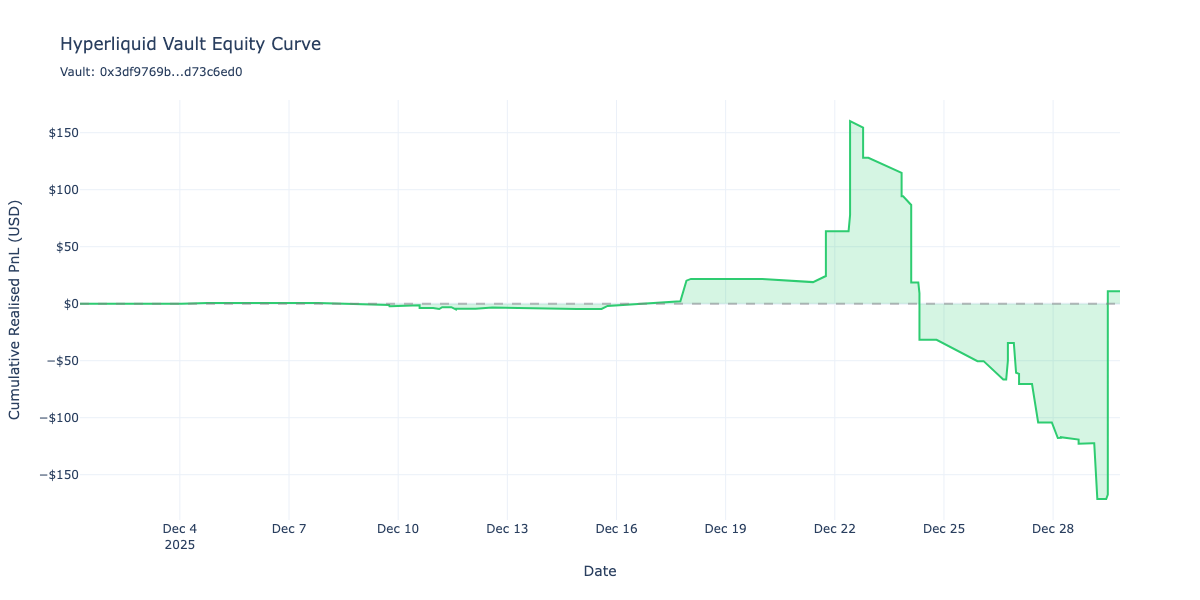
Visualise profit and loss
The equity curve shows how the vault’s cumulative realised PnL evolves over time. This is the key metric for evaluating trading performance.
We use Plotly for interactive visualisation (rendered as static image in documentation).
Note: This profit and loss does not account for vault deposits.
[35]:
# Create equity curve chart
fig = go.Figure()
fig.add_trace(go.Scatter(
x=df.index,
y=df['total_pnl'],
mode='lines',
name='Cumulative PnL',
line=dict(color='#2ecc71', width=2),
fill='tozeroy',
fillcolor='rgba(46, 204, 113, 0.2)',
))
# Add zero line
fig.add_hline(y=0, line_dash="dash", line_color="grey", opacity=0.5)
fig.update_layout(
title=f"Hyperliquid Vault Equity Curve<br><sub>Vault: {VAULT_ADDRESS[:10]}...{VAULT_ADDRESS[-8:]}</sub>",
xaxis_title="Date",
yaxis_title="Cumulative Realised PnL (USD)",
template="plotly_white",
hovermode="x unified",
yaxis=dict(tickformat="$,.0f"),
)
fig.show()
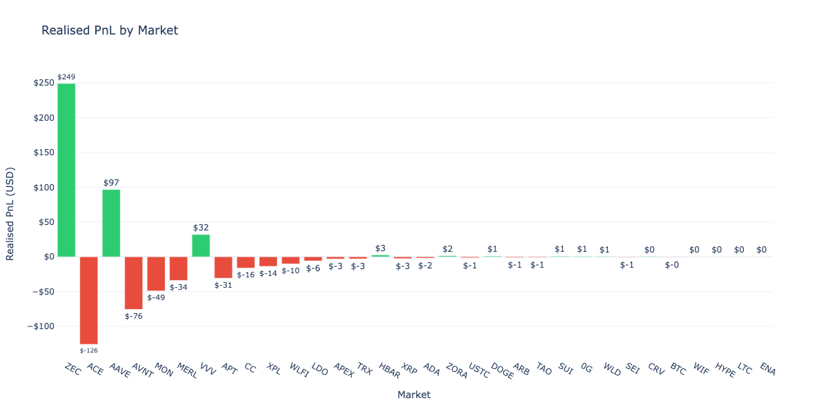
Per-Market PnL Breakdown
Let’s visualise the PnL contribution from each market to understand which assets drove performance.
[36]:
# Calculate total PnL per market (combining long and short)
markets = set(col.rsplit('_', 2)[0] for col in pnl_columns)
market_pnl = {}
for market in markets:
long_col = f"{market}_long_pnl"
short_col = f"{market}_short_pnl"
total = 0
if long_col in df.columns:
total += df[long_col].iloc[-1]
if short_col in df.columns:
total += df[short_col].iloc[-1]
market_pnl[market] = total
# Sort by absolute PnL
sorted_markets = sorted(market_pnl.items(), key=lambda x: abs(x[1]), reverse=True)
# Create bar chart
fig = go.Figure()
colours = ['#2ecc71' if pnl >= 0 else '#e74c3c' for _, pnl in sorted_markets]
fig.add_trace(go.Bar(
x=[m[0] for m in sorted_markets],
y=[m[1] for m in sorted_markets],
marker_color=colours,
text=[f"${pnl:,.0f}" for _, pnl in sorted_markets],
textposition='outside',
))
fig.update_layout(
title="Realised PnL by Market",
xaxis_title="Market",
yaxis_title="Realised PnL (USD)",
template="plotly_white",
yaxis=dict(tickformat="$,.0f"),
)
fig.show()
Vault deposits and withdrawals
Hyperliquid vaults track capital flows through deposits and withdrawals. Understanding these flows is crucial for analysing vault performance in context:
Deposits: Capital added by followers/investors
Withdrawals: Capital removed by followers (subject to lockup periods)
Net flow: Deposits minus withdrawals indicates investor sentiment
We use the userNonFundingLedgerUpdates API endpoint to fetch these events.
[37]:
from eth_defi.hyperliquid.deposit import fetch_vault_deposits, create_deposit_dataframe, get_deposit_summary
# Fetch deposit/withdrawal events for the vault
deposit_events = list(fetch_vault_deposits(
session,
VAULT_ADDRESS,
start_time=START_TIME,
end_time=END_TIME,
))
print(f"Fetched {len(deposit_events)} deposit/withdrawal events")
# Create DataFrame for analysis
deposits_df = create_deposit_dataframe(deposit_events)
# Show summary statistics
summary = get_deposit_summary(deposit_events)
summary_table = pd.DataFrame({
"Metric": [
"Total Events",
"Deposits",
"Withdrawals",
"Total Deposited (USD)",
"Total Withdrawn (USD)",
"Net Flow (USD)",
],
"Value": [
summary["total_events"],
summary["deposits"],
summary["withdrawals"],
f"${float(summary['total_deposited']):,.2f}",
f"${float(summary['total_withdrawn']):,.2f}",
f"${float(summary['net_flow']):,.2f}",
]
})
display(summary_table.set_index("Metric"))
# Show individual events
if not deposits_df.empty:
display(deposits_df[["event_type", "usdc"]].head(10))
Fetched 9 deposit/withdrawal events
| Value | |
|---|---|
| Metric | |
| Total Events | 9 |
| Deposits | 9 |
| Withdrawals | 0 |
| Total Deposited (USD) | $4,650.00 |
| Total Withdrawn (USD) | $0.00 |
| Net Flow (USD) | $4,650.00 |
| event_type | usdc | |
|---|---|---|
| timestamp | ||
| 2025-12-12 00:49:31.304 | vault_deposit | 5.00 |
| 2025-12-12 11:22:01.764 | vault_deposit | 5.00 |
| 2025-12-14 05:03:02.056 | vault_deposit | 500.00 |
| 2025-12-15 14:51:27.419 | vault_deposit | 1,000.00 |
| 2025-12-18 16:25:59.419 | vault_deposit | 100.00 |
| 2025-12-18 16:29:23.102 | vault_deposit | 1,000.00 |
| 2025-12-22 15:27:58.562 | vault_deposit | 1,000.00 |
| 2025-12-23 12:33:40.758 | vault_deposit | 40.00 |
| 2025-12-29 20:28:58.122 | vault_deposit | 1,000.00 |
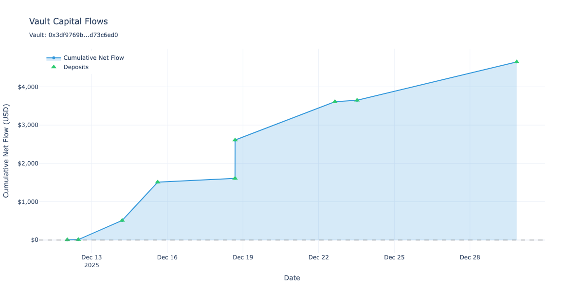
Visualise cumulative capital flows
This chart shows how capital has flowed into and out of the vault over time. A rising line indicates net inflows (more deposits than withdrawals), while a falling line indicates net outflows.
[38]:
if not deposits_df.empty:
# Calculate cumulative flows
deposits_df["cumulative_flow"] = deposits_df["usdc"].cumsum()
# Create the chart
fig = go.Figure()
# Add cumulative flow line
fig.add_trace(go.Scatter(
x=deposits_df.index,
y=deposits_df["cumulative_flow"],
mode="lines+markers",
name="Cumulative Net Flow",
line=dict(color="#3498db", width=2),
fill="tozeroy",
fillcolor="rgba(52, 152, 219, 0.2)",
))
# Add individual events as markers
deposit_mask = deposits_df["event_type"] == "vault_deposit"
withdraw_mask = deposits_df["event_type"] == "vault_withdraw"
if deposit_mask.any():
fig.add_trace(go.Scatter(
x=deposits_df[deposit_mask].index,
y=deposits_df[deposit_mask]["cumulative_flow"],
mode="markers",
name="Deposits",
marker=dict(color="#2ecc71", size=10, symbol="triangle-up"),
text=[f"${v:,.0f}" for v in deposits_df[deposit_mask]["usdc"]],
hovertemplate="%{text}<extra>Deposit</extra>",
))
if withdraw_mask.any():
fig.add_trace(go.Scatter(
x=deposits_df[withdraw_mask].index,
y=deposits_df[withdraw_mask]["cumulative_flow"],
mode="markers",
name="Withdrawals",
marker=dict(color="#e74c3c", size=10, symbol="triangle-down"),
text=[f"${abs(v):,.0f}" for v in deposits_df[withdraw_mask]["usdc"]],
hovertemplate="%{text}<extra>Withdrawal</extra>",
))
fig.add_hline(y=0, line_dash="dash", line_color="grey", opacity=0.5)
fig.update_layout(
title=f"Vault Capital Flows<br><sub>Vault: {VAULT_ADDRESS[:10]}...{VAULT_ADDRESS[-8:]}</sub>",
xaxis_title="Date",
yaxis_title="Cumulative Net Flow (USD)",
template="plotly_white",
hovermode="x unified",
yaxis=dict(tickformat="$,.0f"),
legend=dict(yanchor="top", y=0.99, xanchor="left", x=0.01),
)
fig.show()
else:
print("No deposit/withdrawal events in the selected time period")
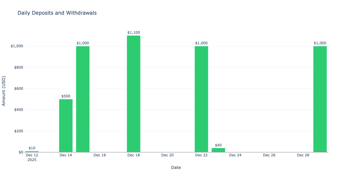
Daily deposit and withdrawal bar chart
This chart shows the daily breakdown of deposits (green, positive) and withdrawals (red, negative) to identify patterns in investor behaviour.
[39]:
if not deposits_df.empty:
# Aggregate by date
deposits_df["date"] = deposits_df.index.date
# Separate deposits and withdrawals
daily_deposits = deposits_df[deposits_df["usdc"] > 0].groupby("date")["usdc"].sum()
daily_withdrawals = deposits_df[deposits_df["usdc"] < 0].groupby("date")["usdc"].sum()
# Create figure with bars
fig = go.Figure()
if not daily_deposits.empty:
fig.add_trace(go.Bar(
x=daily_deposits.index,
y=daily_deposits.values,
name="Deposits",
marker_color="#2ecc71",
text=[f"${v:,.0f}" for v in daily_deposits.values],
textposition="outside",
))
if not daily_withdrawals.empty:
fig.add_trace(go.Bar(
x=daily_withdrawals.index,
y=daily_withdrawals.values,
name="Withdrawals",
marker_color="#e74c3c",
text=[f"${abs(v):,.0f}" for v in daily_withdrawals.values],
textposition="outside",
))
fig.add_hline(y=0, line_color="grey", opacity=0.5)
fig.update_layout(
title="Daily Deposits and Withdrawals",
xaxis_title="Date",
yaxis_title="Amount (USD)",
template="plotly_white",
barmode="relative",
yaxis=dict(tickformat="$,.0f"),
legend=dict(yanchor="top", y=0.99, xanchor="right", x=0.99),
)
fig.show()
else:
print("No deposit/withdrawal events in the selected time period")
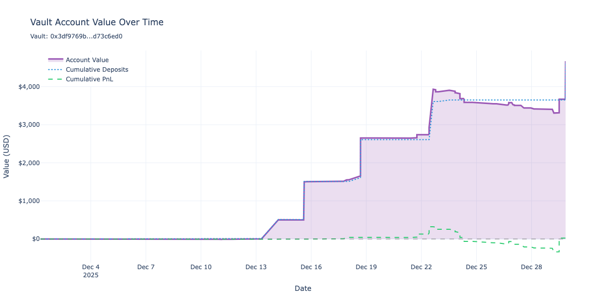
Account value
The previous sections analysed trading PnL and capital flows separately. To understand the true vault performance, we need to combine both into a single account value metric that tracks:
Cumulative PnL: Realised profit/loss from trading activity
Cumulative Net Flow: Total capital deposited minus withdrawn
Account Value: The sum of initial balance, net flows, and trading PnL
This combined view shows how the vault’s total value evolves over time, accounting for both trading performance and capital movements.
We use the analyse_positions_and_deposits() function to merge the position and deposit timelines into a unified DataFrame.
[40]:
from eth_defi.hyperliquid.combined_analysis import analyse_positions_and_deposits, get_combined_summary
# Combine position and deposit data into unified timeline
combined_df = analyse_positions_and_deposits(df, deposits_df)
# Show summary statistics
summary = get_combined_summary(combined_df)
summary_table = pd.DataFrame({
"Metric": [
"Total Events",
"Trading PnL",
"Net Capital Flow",
"Final Account Value",
"Max Account Value",
"Min Account Value",
"Max Drawdown",
],
"Value": [
summary["total_events"],
f"${summary['total_pnl']:,.2f}",
f"${summary['total_netflow']:,.2f}",
f"${summary['final_account_value']:,.2f}",
f"${summary['max_account_value']:,.2f}",
f"${summary['min_account_value']:,.2f}",
f"${summary['max_drawdown']:,.2f}",
]
})
display(summary_table.set_index("Metric"))
# Show the combined DataFrame
display(combined_df.tail())
| Value | |
|---|---|
| Metric | |
| Total Events | 138 |
| Trading PnL | $21.70 |
| Net Capital Flow | $4,650.00 |
| Final Account Value | $4,671.70 |
| Max Account Value | $4,671.70 |
| Min Account Value | $-9.94 |
| Max Drawdown | $-623.16 |
| pnl_update | netflow_update | cumulative_pnl | cumulative_netflow | cumulative_account_value | total_assets | total_supply | share_price | |
|---|---|---|---|---|---|---|---|---|
| timestamp | ||||||||
| 2025-12-29 20:07:28.020 | 0.00 | 0.00 | 21.70 | 3,650.00 | 3,671.70 | 3,671.70 | 3,468.21 | 1.06 |
| 2025-12-29 20:07:28.020 | 0.00 | 0.00 | 21.70 | 3,650.00 | 3,671.70 | 3,671.70 | 3,468.21 | 1.06 |
| 2025-12-29 20:07:28.020 | 0.00 | 0.00 | 21.70 | 3,650.00 | 3,671.70 | 3,671.70 | 3,468.21 | 1.06 |
| 2025-12-29 20:07:28.020 | 0.00 | 0.00 | 21.70 | 3,650.00 | 3,671.70 | 3,671.70 | 3,468.21 | 1.06 |
| 2025-12-29 20:28:58.122 | 0.00 | 1,000.00 | 21.70 | 4,650.00 | 4,671.70 | 4,671.70 | 4,412.79 | 1.06 |
Visualise account value over time
This chart shows the vault’s total account value evolution, combining both trading PnL and capital flows. The account value line represents what the vault would be worth at each point in time.
[41]:
if not combined_df.empty:
fig = go.Figure()
# Add account value line
fig.add_trace(go.Scatter(
x=combined_df.index,
y=combined_df["cumulative_account_value"],
mode="lines",
name="Account Value",
line=dict(color="#9b59b6", width=3),
fill="tozeroy",
fillcolor="rgba(155, 89, 182, 0.2)",
))
# Add cumulative net flow line for reference
fig.add_trace(go.Scatter(
x=combined_df.index,
y=combined_df["cumulative_netflow"],
mode="lines",
name="Cumulative Deposits",
line=dict(color="#3498db", width=2, dash="dot"),
))
# Add cumulative PnL line for reference
fig.add_trace(go.Scatter(
x=combined_df.index,
y=combined_df["cumulative_pnl"],
mode="lines",
name="Cumulative PnL",
line=dict(color="#2ecc71", width=2, dash="dash"),
))
fig.add_hline(y=0, line_dash="dash", line_color="grey", opacity=0.5)
fig.update_layout(
title=f"Vault Account Value Over Time<br><sub>Vault: {VAULT_ADDRESS[:10]}...{VAULT_ADDRESS[-8:]}</sub>",
xaxis_title="Date",
yaxis_title="Value (USD)",
template="plotly_white",
hovermode="x unified",
yaxis=dict(tickformat="$,.0f"),
legend=dict(yanchor="top", y=0.99, xanchor="left", x=0.01),
)
fig.show()
else:
print("No data available for account value visualisation")
Share price
Unlike ERC-4626 vaults that have native share tokens, Hyperliquid vaults don’t provide an on-chain share price mechanism. However, we can calculate an internal share price using the same principles:
Total assets: The vault’s net asset value (NAV) at any point in time
Total supply: The number of virtual shares outstanding
Share price: Calculated as
total_assets / total_supply
The share price mechanism works as follows:
Share price starts at $1.00 when the first deposit occurs
Deposits mint new shares at the current share price:
shares_minted = deposit_amount / share_priceWithdrawals burn shares at the current share price:
shares_burned = withdrawal_amount / share_priceTrading PnL changes total assets but not total supply, which changes the share price
This allows us to measure true investment performance independent of capital flows. If share price increases, depositors are making money; if it decreases, they’re losing money—regardless of when they deposited.
[42]:
# Display share price metrics from the combined analysis
# The combined_df already has share price columns calculated
if not combined_df.empty and "share_price" in combined_df.columns:
# Show share price summary statistics
summary = get_combined_summary(combined_df)
share_price_table = pd.DataFrame({
"Metric": [
"Initial Share Price",
"Final Share Price",
"Share Price Change",
"Final Total Supply (shares)",
"Final Total Assets (USD)",
],
"Value": [
"$1.00",
f"${summary['final_share_price']:.4f}",
f"{summary['share_price_change'] * 100:+.2f}%",
f"{summary['final_total_supply']:,.2f}",
f"${summary['final_account_value']:,.2f}",
]
})
display(share_price_table.set_index("Metric"))
# Show share price data from the DataFrame
display(combined_df[["total_assets", "total_supply", "share_price"]].head(10))
display(combined_df[["total_assets", "total_supply", "share_price"]].tail(10))
else:
print("Share price data not available")
| Value | |
|---|---|
| Metric | |
| Initial Share Price | $1.00 |
| Final Share Price | $1.0587 |
| Share Price Change | +0.00% |
| Final Total Supply (shares) | 4,412.79 |
| Final Total Assets (USD) | $4,671.70 |
| total_assets | total_supply | share_price | |
|---|---|---|---|
| timestamp | |||
| 2025-12-01 06:07:19.756 | 0.00 | 0.00 | 1.00 |
| 2025-12-02 11:01:08.209 | 0.00 | 0.00 | 1.00 |
| 2025-12-03 22:05:03.025 | 0.00 | 0.00 | 1.00 |
| 2025-12-04 01:01:07.787 | 0.00 | 0.00 | 1.00 |
| 2025-12-04 18:01:21.837 | 1.37 | 0.00 | 1.00 |
| 2025-12-04 21:01:23.198 | 1.37 | 0.00 | 1.00 |
| 2025-12-05 00:01:58.248 | 1.37 | 0.00 | 1.00 |
| 2025-12-07 18:12:28.519 | 1.37 | 0.00 | 1.00 |
| 2025-12-07 19:04:41.073 | 1.37 | 0.00 | 1.00 |
| 2025-12-09 18:03:36.373 | -2.37 | 0.00 | 1.00 |
| total_assets | total_supply | share_price | |
|---|---|---|---|
| timestamp | |||
| 2025-12-29 12:05:01.984 | 3,314.94 | 3,468.21 | 0.96 |
| 2025-12-29 12:05:01.984 | 3,606.72 | 3,468.21 | 1.04 |
| 2025-12-29 12:05:01.984 | 3,671.70 | 3,468.21 | 1.06 |
| 2025-12-29 13:05:31.428 | 3,671.70 | 3,468.21 | 1.06 |
| 2025-12-29 13:05:31.428 | 3,671.70 | 3,468.21 | 1.06 |
| 2025-12-29 20:07:28.020 | 3,671.70 | 3,468.21 | 1.06 |
| 2025-12-29 20:07:28.020 | 3,671.70 | 3,468.21 | 1.06 |
| 2025-12-29 20:07:28.020 | 3,671.70 | 3,468.21 | 1.06 |
| 2025-12-29 20:07:28.020 | 3,671.70 | 3,468.21 | 1.06 |
| 2025-12-29 20:28:58.122 | 4,671.70 | 4,412.79 | 1.06 |
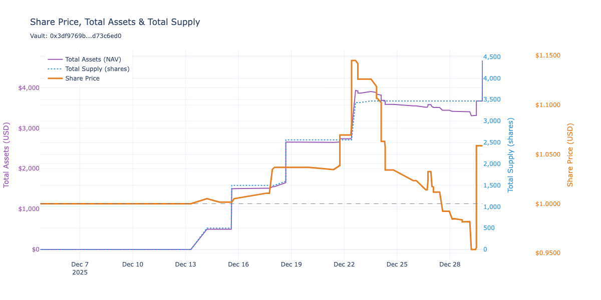
Visualise share price, total assets and total supply
This chart shows the vault’s share price evolution alongside total assets (NAV) and total supply (shares outstanding). The share price is the most important metric for evaluating investment performance—it shows what return depositors are getting independent of capital flows.
Share price (orange): Investment performance metric, starts at $1.00
Total assets (purple): The vault’s net asset value (NAV)
Total supply (blue): Number of shares outstanding
When total assets grow faster than total supply (due to trading profits), share price increases. When assets shrink relative to supply (due to losses), share price decreases.
[43]:
if not combined_df.empty and "share_price" in combined_df.columns:
# Filter to rows where shares exist (share price is meaningful)
# This removes any events before the first deposit
share_data = combined_df[combined_df["total_assets"] > 0].copy()
# Find the first timestamp where shares exist and filter from there
if not share_data.empty:
first_share_timestamp = share_data.index.min()
share_data = share_data.loc[first_share_timestamp:]
if not share_data.empty:
from plotly.subplots import make_subplots
# Create figure with three y-axes
fig = make_subplots(specs=[[{"secondary_y": True}]])
# Add total assets line (left y-axis)
fig.add_trace(
go.Scatter(
x=share_data.index,
y=share_data["total_assets"],
mode="lines",
name="Total Assets (NAV)",
line=dict(color="#9b59b6", width=2),
),
secondary_y=False,
)
# Add total supply line (right y-axis)
fig.add_trace(
go.Scatter(
x=share_data.index,
y=share_data["total_supply"],
mode="lines",
name="Total Supply (shares)",
line=dict(color="#3498db", width=2, dash="dot"),
),
secondary_y=True,
)
# Add share price line on a third axis (overlaid on right side)
fig.add_trace(
go.Scatter(
x=share_data.index,
y=share_data["share_price"],
mode="lines",
name="Share Price",
line=dict(color="#e67e22", width=3),
yaxis="y3",
),
)
# Add reference line at $1.00 (initial share price) on the third axis
fig.add_shape(
type="line",
x0=share_data.index.min(),
x1=share_data.index.max(),
y0=1.0,
y1=1.0,
yref="y3",
line=dict(color="grey", width=1, dash="dash"),
)
fig.update_layout(
title=f"Share Price, Total Assets & Total Supply<br><sub>Vault: {VAULT_ADDRESS[:10]}...{VAULT_ADDRESS[-8:]}</sub>",
xaxis=dict(domain=[0, 0.85]), # Shrink x-axis to make room for right axes
template="plotly_white",
hovermode="x unified",
legend=dict(yanchor="top", y=0.99, xanchor="left", x=0.01),
# Configure third y-axis for share price (positioned further right)
yaxis3=dict(
title=dict(text="Share Price (USD)", font=dict(color="#e67e22")),
tickfont=dict(color="#e67e22"),
tickformat="$,.4f",
anchor="free",
overlaying="y",
side="right",
position=0.95,
),
# Adjust margins to accommodate third axis
margin=dict(r=80),
)
fig.update_yaxes(
title=dict(text="Total Assets (USD)", font=dict(color="#9b59b6")),
tickformat="$,.0f",
tickfont=dict(color="#9b59b6"),
secondary_y=False,
)
fig.update_yaxes(
title=dict(text="Total Supply (shares)", font=dict(color="#3498db")),
tickformat=",.0f",
tickfont=dict(color="#3498db"),
secondary_y=True,
anchor="x",
)
fig.show()
else:
print("No share price data available (no deposits yet)")
else:
print("Share price data not available")